Real estate economics

Real estate economics is the application of economic techniques to real estate markets. It tries to describe, explain, and predict patterns of real estate prices, building production, and real estate consumption. The closely related field of housing economics is narrower in scope, concentrating on residential real estate markets. Both draw on partial equilibrium analysis (supply and demand), urban economics, spatial economics, and finance.

Overview of real estate markets

The main participants in real estate markets are:

• Owner/User - These people are both owners and tenants. They purchase houses as an investment and also to live in.
• Owner - These people are pure investors. They do not consume the real estate that they purchase. Typically they rent out the property to someone else.
• Renter - These people are pure consumers.
• Developers - These people prepare raw land for building which results in new product for the market.
• Renovators - These people supply refurbished buildings to the market.
• Facilitators - This includes banks, real estate brokers, lawyers, and others that facilitate the purchase and sale of real estate.

The owner/user, owner, and renter comprise the demand side of the market, while the developers and renovators comprise the supply side. In order to apply simple supply and demand analysis to real estate markets a number of modification need to be made to standard microeconomic assumptions and procedures. In particular, the unique characteristics of the real estate market must be accommodated. These characteristics include:

• Durability - Real estate is durable. A building can last for decades or even centuries, and the land underneath it is practically indestructible. Because of this, real estate markets are modeled as a stock/flow market. About 98% of supply consists of the stock of existing houses, while about 2% consists of the flow of new development. The stock of real estate supply in any period, is determined by the existing stock in the previous period, the rate of deterioration of the existing stock, the rate of renovation of the existing stock, and the flow of new development in the current period. The effect of real estate market adjustments tend to be mitigated by the relatively large stock of existing buildings.
• Heterogeneous - Every piece of real estate is unique, in terms of its location, in terms of the building, and in terms of its financing. This makes pricing difficult, increases search costs, creates information asymmetry and greatly restricts substitutability. To get around this problem economists (beginning with Muth (1960)) define supply in terms of service units, that is, any physical unit can be deconstructed into the services that it provides. Olsen (1969) describes these units of housing services as an unobservable theoretical construct. Housing stock depreciates making it qualitatively different from a new building. The market equilibriating process operates across multiple quality levels. Further, the real estate market is typically divided into residential, commercial, and industrial segments. It can also be further divided into subcategories like recreational, income generating, area, historical/protected, etc.
• High Transaction costs - Buying and/or moving into a home cost much more than most types of transactions. These costs include search costs, real estate fees, moving costs, legal fees, land transfer taxes, and deed registration fees. Transaction costs for the seller typically range between 8 - 10 % of the purchase price.
• Long time delays - The market adjustment process is subject to time delays due to the length of time it takes to finance, design, and construct new supply, and also due to the relatively slow rate of change of demand. Because of these lags there is a great potential for disequilibrium in the short run. Adjustment mechanisms tend to be slow, relative to more fluid markets.
• Both an investment good and a consumption good - Real estate can be purchased with the expectation of attaining a return (an investment good), or with the intention of using it (a consumption good), or both. These functions can be separated (with market participants concentrating on one or the other function) or can be combined (in the case of the person that lives in a house that they own). This dual nature of the good means that it is not uncommon for people to over-invest in real estate, that is, to invest more money in an asset than it is worth on the open market.
• Immobility - Real estate is locationaly immobile. Consumers come to the good rather than the good going to the consumer. Because of this, there can be no physical market-place. This spatial fixity means that market adjustment must occur by people moving to dwelling units, rather than the movement of the goods. For example, if tastes change and more people demand suburban houses, people must find housing in the suburbs, because it is impossible to bring their existing house to the suburb. Spatial fixity combined with the close proximity of housing units in urban areas suggest the potential for externalities inherent in a given location.

Demand for housing

The main determinants of the demand for housing are demographic. However other factors like income, price of housing, cost and availability of credit, consumer preferences, investor preferences, price of substitutes and price of compliments all play a role.

The core demographic variables are population size and population growth : the more people in the economy, the greater the demand for housing. But this is an oversimplification. It is necessary to consider family size, the age composition of the family, the number of first and second children, net migration (immigration minus emigration), non-family household formation, the number of double family households, death rates, divorce rates, and marriages. In housing economics, the elemental unit of analysis is not the individual as it is in standard partial equilibrium models. Rather, it is households that demand housing services: typically one household per house. The size and demographic composition of households is variable and not entirely exogenous. It is endogenous to the housing market in the sense that as the price of housing services increase, household size will tend also to increase.

Income is also an important determinant. Empirical measures of the income elasticity of demand in North America range from 0.5 to 0.9 (De Leeuw, F. 1971). If permanent income elasticity is measured, the results are a little higher (Kain and Quigley 1975) because transitory income varies from year-to-year and across individuals so positive transitory income will tend to cancel out negative transitory income. Many housing economists use permanent income rather than annual income because of the high cost of purchasing real estate. For many people, real estate will be the most costly item they will ever buy.

The price of housing is also an important factor. The price elasticity of the demand for housing services in North America is estimated as negative 0.7 by Polinsky and Ellwood (1979), and as negative 0.9 by Maisel, Burnham, and Austin (1971).

An individual household’s housing demand can be modeled with standard utility/choice theory. A utility function, such as U=U(X1,X2,X3,X4,...Xn), can be constructed in which the households utility is a function of various goods and services (Xs). This will be subject to a budget constraint such as P1X1+P2X2+...PnXn=Y, where Y is the households available income and the Ps are the prices for the various goods and services. The equality indicates that the money spent on all the goods and services must be equal to the available income. Because this is unrealistic, the model must be adjusted to allow for borrowing and/or saving. A measure of wealth, lifetime income, or permanent income is required. The model must also be adjusted to account for the heterogeneousness of real estate. This can be done by deconstructing the utility function. If housing services (X4) is separated into the components that comprise it (Z1,Z2,Z3,Z4,...Zn), then the utility function can be rewritten as U=U(X1,X2,X3,(Z1,Z2,Z3,Z4,...Zn)...Xn) By varying the price of housing services (X4) and solving for points of optimal utility, that household's demand schedule for housing services can be constructed. Market demand is calculated by summing all individual household demands.

Supply of housing

Housing supply is produced using land, labour, and various inputs such as electricity and building materials. The quantity of new supply is determined by the cost of these inputs, the price of the existing stock of houses, and the technology of production. For a typical single family dwelling in suburban North America, approximate percentage costs can be broken down as: acquisition costs 10%, site improvement costs 11%, labour costs 26%, materials costs 31%, finance costs 3%, administrative costs 15%, and marketing costs 4%. Multi-unit residential dwellings typically break down as: acquisition costs 7%, site improvement costs 8%, labour costs 27%, materials costs 33%, finance costs 4%, administrative costs 17%, and marketing costs 5%. Public subdivision requirements can increase development cost by up to 3% depending on the jurisdiction. Differences in building codes account for about a 2% variation in development costs. However these subdivision and building code costs typically increase the market value of the buildings by at least the amount of their cost outlays. A production function such as Q=f(L,N,M) can be constructed in which Q is the quantity of houses produced, N is the amount of labour employed, L is the amount of land used, and M is the amount of other materials. This production function must, however, be adjusted to account for the refurbishing and augmentation of existing buildings. To do this a second production function is constructed that includes the stock of existing housing, and their ages, as determinants. The two functions are summed yielding the total production function. Alternatively an hedonic pricing model can be regressed.

The long-run price elasticity of supply is quite high. George Fallis estimates it as 8.2 (Fallis, G. 1985), but in the short run supply tends to be very price inelastic. Supply price elasticity depends on the elasticity of substitution and supply restrictions. There is significant substitutability both between land and materials, and between labour and materials. In high value locations, multi-story concrete building are typically built to reduce the amount of expensive land used. As labour costs increased since the 1950s, new materials and capital intensive techniques have been employed to reduce the amount of relatively expensive labour used. However supply restrictions can significantly effect substitutability. In particular the lack of supply of skilled labour (and labour union requirements), can constrain the substitution from capital to labour. Land availability can also constrain substitutability if the area of interest is delineated (that is, the larger the area, the more suppliers of land, and the more substitution that is possible). Land use controls such as zoning bylaws can also reduce land substitutability.

The adjustment mechanism

The basic adjustment mechanism is a stock/flow model to reflect the fact that about 98% the market is comprised of existing stock and about 2% consists of the flow of new buildings.

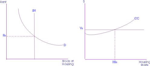
In the diagram to the right, the stock of housing supply is presented in the left panel while the new flow is in the right panel. There are four steps in the basic adjustment mechanism. First, the initial equilibrium price (Ro) is determined by the intersection of the supply of existing housing stock (SH) and the demand for housing (D). This rent is then translated into value (Vo) via discounting cash flows. Value is calculated by dividing current period rents by the discount rate, that is, as a perpetuity. Then value is compared to construction costs (CC) in order to determine whether profitable opportunities exist for developers. The intersection of construction costs and the value of housing services determine the maximum level of new housing starts (HSo). Finally the amount of housing starts in the current period is added to the available stock of housing in the next period. In the next period, supply curve SH will shift to the right by amount HSo.

Adjustment with depreciation

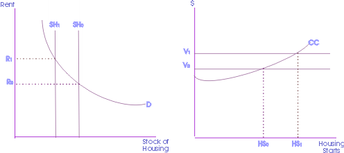
The diagram to the left shows the effects of depreciation. If the supply of existing housing deteriates due to wear, then the stock of housing supply depreciates. Because of this, the supply of housing (SHo) will shift to the left (to SH1) resulting in a new equilibrium price of R1. The increase of prices from Ro to R1 will shift the value function up (from Vo to V1). As a result, more houses can be produced profitably and housing starts will increase (from HSo to HS1). Then the supply of housing will shift back to its initial position (SH1 to SHo).

Increase in demand

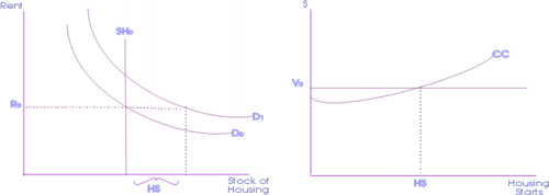
The diagram on the right shows the effects of an increase in demand in the short run. If there is an increase in the demand for housing, such as the shift from Do to D1 there will be either a price or quantity adjustment, or both. For the price to stay the same, the supply of housing must increase. That is, supply SHo must increase by HS.

Increase in costs

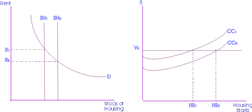
The diagram on the left shows the effects of an increase in costs in the short-run. If construction costs increase (say from CCo to CC1), developers will find their business less profitable and will be more selective in their ventures. In addition some developers may leave the industry. The quantity of housing starts will decrease (HSo to HS1). This will eventually reduce the level of supply (from SHo to SH1) as the existing stock of housing depreciates. Prices will tend to rise (from Ro to R1).

References

• Bourne, L.S. and Hitchcock, J.R. editors., (1978) Urban Housing Markets :Recent directions in research and policy, University of Toronto Press, Toronto, 1978.
• De Leeuw, F. (1971) The demand for housing, A review of the cross-sectional evidence, Review of Economics and Statistics, vol. 53, no. 1, pp. 1-10.
• Fallis, G. (1985) Housing Economics, Butterworth, Toronto, 1985.
• Kain J.F. and Quigley J.M. (1975) Housing Markets and Racial Discrimination, National Bureau of Economic Research, New York.
• Maisel S.J., Burnham J.B., and Austin J.S. (1971) The demand for housing, Review of Economics and Statistics, Vol. 53, pp. 410-413.
• Muth, R. (1960) “The demand for non-farm housingâ€�, in A.C.Harberger, ed., The demand for durable goods, University of Chicago Press, Chicago, 1960.
• Olsen, E.O. (1969) “A competitive theory of the housing marketâ€�, American Economic Review, Vol. 59, pp. 612-622.
• Polinsky A. M. and Ellwood D.T. (1979) An empirical reconciliation of micro and group estimates of the demand for housing, Review of Economics and Statistics, vol. 61, pp. 199-205.